Derive the Fourier Series Expansion for Each of the Following Continuoustime Signals

Derivation of Fourier Series

The previous page showed that a time domain signal can be represented as a sum of sinusoidal signals (i.e., the frequency domain), but the method for determining the phase and magnitude of the sinusoids was not discussed. This page will describe how to determine the frequency domain representation of the signal. For now we will consider only periodic signals, though the concept of the frequency domain can be extended to signals that are not periodic (using what is called the Fourier Transform). The next page will give several examples.

Contents

Statement of the Problem

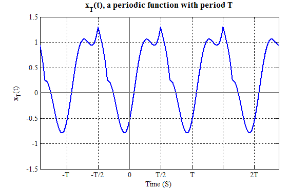
Consider a periodic signal x_T(t) with period T (we will write periodic signals with a subscript corresponding to the period). Since the period is T, we take the fundamental frequency to be ω₀=2π/T. We can represent any such function (with some very minor restrictions) using Fourier Series.

In the early 1800's Joseph Fourier determined that such a function can be represented as a series of sines and cosines. In other words he showed that a function such as the one above can be represented as a sum of sines and cosines of different frequencies, called a Fourier Series. There are two common forms of the Fourier Series, "Trigonometric" and "Exponential." These are discussed below, followed by a demonstration that the two forms are equivalent. For easy reference the two forms are stated here, their derivation follows.

$$
\begin{align}
x\left( t \right) &= a_0 + \sum\limits_{n = 1}^\infty {\left( {a_n \cos \left( {n\omega _0 t} \right) + b_n \sin \left( {n\omega _0 t} \right)} \right)} \quad \quad Trigonometric \ Form\cr
&= \sum\limits_{n = - \infty }^\infty {c_n e^{jn\omega _0 t} } \quad \quad \quad \quad\quad \quad \quad \quad Exponential \ Form\end{align}
$$

The Trigonometric Series

The Fourier Series is more easily understood if we first restrict ourselves to functions that are either even or odd. We will then generalize to any function.

Aside: Even and Odd functions

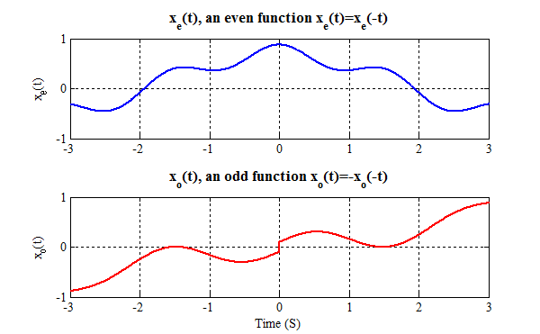
The following derivations require some knowledge of even and odd functions, so a brief review is presented. An even function, x_e(t), is symmetric about t=0, so x_e(t)=x_e(-t). An odd function, x_o(t), is antisymmetric about t=0, so x_o(t)=-x_o(-t) (note: this implies that x_o(0)=0 ). Examples are shown below.

Other important facts about even and odd functions:

1. the product of two even functions is an even function. Given two even functions x_e1(t) and x_e2(t), their product y_e(t)=x_e1(t) · x_e2(t) is even.
   
2. the product of two odd functions is an even function. Given two odd functions x_o1(t) and x_o2(t), their product y_e(t)=x_o1(t)·x_o2(t) is even.
3. the product of an even function and an odd function is an odd function. Given an even function, x_e(t) and an odd function x_o(t), their product y_o(t)=x_e(t)·x_o(t) is odd.
4. the integral of an odd function, x_o(t), from t=-a to t=a is equal to zero
   $$ \int_{ - a}^a {x_o \left( t \right)dt} = 0 $$
5. The same is not generally true of even functions. In other words, the integral of an even function, x_e(t), from t=-a to t=a is not in general equal to zero (but may be in some cases, for example the cosine function)
6. Recall that a cosine is an even function and sine is odd.

Even Functions

An even function, x_e(t), can be represented as a sum of cosines of various frequencies via the equation:

$$ x_e (t) = \sum\limits_{n = 0}^\infty {a_n \cos \left( {n\omega _0 t} \right)} $$

Since cos(nω₀t)=1 when n=0 the series is more commonly written as

$$ x_e (t) = a_0 + \sum\limits_{n = 1}^\infty {a_n \cos \left( {n\omega _0 t} \right)} $$

This is called the "synthesis" equation because it shows how we create, or synthesize, the function x_e(t) by adding up cosines.

An example will demonstrate exactly how the summation describing the synthesis process works. Consider the following function, x_T and its corresponding values for a_n . This function has T=1 so ω₀=2·π/T=2·π. Note: we have not determined how the a_n are calculated; that derivation follows, that calculation comes later.

The top graph corresponds to a₀ , a constant term. We will show later that this is the average value of the original function (a pulse of width 0.4 and period T=1, so average=0.4). This is often called the average, the DC, or the zero frequency ($n\omega_0=0\cdot\omega_0=0$) component of the Fourier series.
(note: {a₀cos(0·ω₀·t) = a₀ )

The second graph is of a₁cos(ω₀t). Note that it has exactly one oscillation of the cosine in the period, T=1. We call this the 1^st, or fundamental harmonic. The amplitude of this harmonic is given by a₁=0.6055.

The 2^nd harmonic (n=2) has exactly two oscillations in one period, T=1, of the original function, and an amplitude of a₂=0.1871.

The 3rd harmonic (n=3) has exactly three oscillations in one period, T=1, of the original function, and an amplitude of a₃=-0.1247.

...and so on, for increasing values of n.

The right column shows the sum $$ a_0 + \sum\limits_{n = 1}^N {a_n \cos \left( {n\omega _0 t} \right)} $$ for n=0 to 4.

• The topmost graph shows the constant (or average) value determined by a₀=0.4. This value is shown in blue, the original function is shown in red.
• The second graph shows (in blue) the summation with N=1. It is the sum of the constant value plus the 1st harmonic (a₀+a₁cos(ω₀t)). In other words the second graph on the right shows the sum of the first two graphs on the left. With only one harmonic the Fourier sum (blue) already has the character of the original (red) - they are both high in the middle.
• The third graph on the right (which is the sum of the first three graphs on the left) is not much different than the second because the added term. a₂cos(2ω₀t) is not very large. However, careful inspection yields that the third graph (blue) is a better fit to the original function (red) than the previous one.
• The fourth graph on the right (the sum of the first four graphs on the left, (a₀ + a₁cos(ω₀ t) + a₂cos(2ω ₀t) + a₃cos(ω₀t)) and the Fourier sum approximation is even better than before.
• ...and so on, for increasing values of n.

How do we find a_n ?

The example above shows how the harmonics add to approximate the original question, but begs the question of how to find the magnitudes of the a_n . Start with the synthesis equation of the Fourier Series for an even function x_e(t) (note, in this equation, that n≥0).

$$ x_e (t) = \sum\limits_{n = 0}^\infty {a_n \cos ( n\omega _0 t)} $$

Now, without justification we multiply both sides by $\cos(m\omega_0t)$

$$
x_e (t)\cos \left( {m\omega _0 t} \right) = \sum\limits_{n = 0}^\infty {a_n \cos \left( {n\omega _0 t} \right)} \cos \left( {m\omega _0 t} \right)
$$

then integrate over one period (note: the exact interval is unimportant, but we will generally use -T/2 to T/2 or 0 to T, depending on which is more convenient).

$$ \int\limits_T {x_e (t)\cos \left( {m\omega _0 t} \right)dt} = \int\limits_T {\sum\limits_{n = 0}^\infty {a_n \cos \left( {n\omega _0 t} \right)} \cos \left( {m\omega _0 t} \right)dt} $$

Now switch the order of summation and integration on the right hand side, followed by application of the trig identity cos(a)cos(b)=½(cos(a+b)+cos(a-b))

$$ \begin{align}
\int\limits_T {x_e (t)\cos \left( {m\omega _0 t} \right)dt} &= \sum\limits_{n = 0}^\infty {a_n \int\limits_T {\cos \left( {n\omega _0 t} \right)\cos \left( {m\omega _0 t} \right)dt} } \\
& = \sum\limits_{n = 0}^\infty {a_n \int\limits_T {{1 \over 2}\left( {\cos \left( {\left( {m + n} \right)\omega _0 t} \right) + \cos \left( {\left( {m - n} \right)\omega _0 t} \right)} \right)dt} } \\
& = {1 \over 2}\sum\limits_{n = 0}^\infty {a_n \int\limits_T {\left( {\cos \left( {\left( {n + m} \right)\omega _0 t} \right) + \cos \left( {\left( {m - n} \right)\omega _0 t} \right)} \right)dt} }
\end{align}$$

Consider only the cases when m>0, then the function cos((m+n)ω₀t) has exactly (m+n) complete oscillations in the interval of integration, T. When we integrate this function, the result is zero (because we are integrating over an an integer (greater than or equal to one) number of oscillations). This simplifies our result to

$$ \begin{align}
\int\limits_T {x_e (t)\cos \left( {m\omega _0 t} \right)dt} &= \frac{1}
{2}\sum\limits_{n = 0}^\infty {a_n \int\limits_T {\left( {\cos \left( {\left( {n + m} \right)\omega _0 t} \right) + \cos \left( {\left( {m - n} \right)\omega _0 t} \right)} \right)dt} } \\
& = \frac{1}
{2}\sum\limits_{n = 0}^\infty {a_n \left( {\int\limits_T {\cos \left( {\left( {n + m} \right)\omega _0 t} \right)dt} + \int\limits_T {\cos \left( {\left( {m - n} \right)\omega _0 t} \right)dt} } \right)} \\
& = \frac{1}
{2}\sum\limits_{n = 0}^\infty {a_n \int\limits_T {\cos \left( {\left( {m - n} \right)\omega _0 t} \right)dt} }
\end{align}$$

Since cosine is an even function cos((m-n)ω₀t)=cos((n-m)ω₀t) is time varying and has exactly |m-n| complete oscillations in the interval of integration, except when m=n in which case cos((m-n)ω₀ = cos(0) = 1 so

$$ \int\limits_T {\cos \left( {\left( {m - n} \right)\omega _0 t} \right)dt} = \left\{ {\matrix{
{\int\limits_T {\cos \left( {\left( {m - n} \right)\omega _0 t} \right)dt = 0} ,\quad m \ne n} \cr
{\int\limits_T {1 \cdot dt} = T,\quad m = n} \cr} } \right. $$

Now look at the summation again

$$ \int\limits_T {x_e (t)\cos \left( {m\omega _0 t} \right)dt} = {1 \over 2}\sum\limits_{n = 0}^\infty {a_n \int\limits_T {\cos \left( {\left( {m - n} \right)\omega _0 t} \right)dt} } $$

As n goes from 0 to ∞ every term in the summation except when m=n will be zero. So the only term that contributes to the summation is m=n, when the integral equals T. So the entire summation reduces to

$$
\displaylines{ \int\limits_T {x_e (t)\cos \left( {m\omega _0 t} \right)dt} = {1 \over 2}a_m T \cr a_m = {2 \over T}\int\limits_T {x_e (t)\cos \left( {m\omega _0 t} \right)dt} \cr
a_n = {2 \over T}\int\limits_T {x_e (t)\cos \left( {n\omega _0 t} \right)dt} \cr} $$

We switched m to n in the last line since m is just a dummy variable. We now have an expression for a_n , which was our goal.

Aside: Further explanation of previous step

In the text above, the equating of the two terms

$$
a_m T = \sum\limits_{n = 0}^\infty {a_n \int\limits_T {\cos \left( {\left( {m - n} \right)\omega _0 t} \right)dt} }
$$

is often puzzling. To explain it, take m=2 and expand the summation

$$\begin{align}
a_2 T &= \sum\limits_{n = 0}^\infty {a_n \int\limits_T {\cos \left( {\left( {2 - n} \right)\omega _0 t} \right)dt} } \cr
&= a_0 \int\limits_T {\cos \left( {\left( {2 - 0} \right)\omega _0 t} \right)dt} + a_1 \int\limits_T {\cos \left( {\left( {2 - 1} \right)\omega _0 t} \right)dt} + a_2 \int\limits_T {\cos \left( {\left( {2 - 2} \right)\omega _0 t} \right)dt} + a_3 \int\limits_T {\cos \left( {\left( {2 - 3} \right)\omega _0 t} \right)dt} + \cdots \cr
&= a_0 \int\limits_T {\cos \left( {2 \cdot \omega _0 t} \right)dt} + a_1 \int\limits_T {\cos \left( {1 \cdot \omega _0 t} \right)dt} + a_2 \int\limits_T {\cos \left( {0 \cdot \omega _0 t} \right)dt} + a_3 \int\limits_T {\cos \left( { - 1 \cdot \omega _0 t} \right)dt} + \cdots \cr
&= a_0 \int\limits_T {\cos \left( {2 \cdot \omega _0 t} \right)dt} + a_1 \int\limits_T {\cos \left( {1 \cdot \omega _0 t} \right)dt} + a_2 \int\limits_T {dt} + a_3 \int\limits_T {\cos \left( {1 \cdot \omega _0 t} \right)dt} + \cdots
\end{align}$$

In the last line we used the fact that cos(0)=1 and cos(-x)=cos(x). All of the integrals but the third one will go to zero because the integration is over an integer number of oscillations (as will all of the omitted terms). The third integral becomes a₂T, as was expected.

Aside: Orthogonality of functions

(you may skip this if you would like to - it is not necessary to proceed).

In the discussion above we use the fact that

$$
\int\limits_T {\cos \left( {n\omega _0 t} \right)\cos \left( {m\omega _0 t} \right)dt} = \left\{ {\matrix{
{{T\over 2},\quad m = n} \cr
{0,\quad m \ne n} \cr } } \right.
$$

This is called the orthogonality function of the cosine. It is similar to orthogonality of vectors. Consider two vectors and their dot product.

$$
\begin{align}
{\bf{x}} &= \left[ {\matrix{
{x_1 } & {x_2 } & {x_3 } & {x_4 } \cr } } \right]\quad \quad {\bf{y}} = \left[ {\matrix{
{y_1 } & {y_2 } & {y_3 } & y \cr } _4 } \right]\quad \cr
{\bf{x}} \cdot {\bf{y}}& = x_1 y_1 + x_2 y_2 + x_3 y_3 + x_4 y_4 \cr
&= \sum\limits_{i = 1}^N {x_i y_i } \cr\end{align}
$$

We say the vectors x and y are orthogonal if their dot product (the sum the elementwise products of the vectors' elements) is zero. If we switch integral for sum (since the function is a continuous function of time) we say functions are orthogonal if the integral of the product of the two functions is zero.

The derivation of the Fourier series coefficients is not complete because, as part of our proof, we didn't consider the case when m=0. (Note: we didn't consider this case before because we used the argument that cos((m+n)ω₀t) has exactly (m+n) complete oscillations in the interval of integration, T). For the special case m=0

$$
\begin{align}
\int\limits_T {x_e (t)\cos \left( {m\omega _0 t} \right)dt} &= \sum\limits_{n = 0}^\infty {a_n \int\limits_T {\cos \left( {n\omega _0 t} \right)\cos \left( {m\omega _0 t} \right)dt} } \cr
\int\limits_T {x_e (t)\cos \left( {0 \cdot \omega _0 t} \right)dt} &= \sum\limits_{n = 0}^\infty {a_n \int\limits_T {\cos \left( {n\omega _0 t} \right)\cos \left( {0 \cdot \omega _0 t} \right)dt} } \quad \quad {\text{but }}\cos \left( {0 \cdot \omega _0 t} \right) &= 1 \cr
\int\limits_T {x_e (t)dt} &= \sum\limits_{n = 0}^\infty {a_n \int\limits_T {\cos \left( {n\omega _0 t} \right)dt} } \cr
\int\limits_T {x_e (t)dt} &= Ta_0 \end{align}
$$

This leads to the result stated above, that a₀ is the average value of the function

$$ a_0 = \frac{1} {T}\int\limits_T {x_e (t)dt} = {\text{average of x}}_e \left( t \right) $$

Odd Functions

An odd function can be represented by a Fourier Sine series (to represent even functions we used cosines (an even function), so it is not surprising that we use sinusoids.

$$
x_o \left( t \right) = \sum\limits_{n = 1}^\infty {b_n \sin \left( {n\omega _0 t} \right)}
$$

Note that there is no b₀ term since the average value of an odd function over one period is always zero.

The coefficients b_n can be determined from the equation

$$
b_n = \frac2T\int\limits_T {x_o (t)\sin \left( {n\omega _0 t} \right)dt}
$$

The derivation closely follows that for the a_n coefficients.

Arbitrary Functions (not necessarily even or odd)

Any function can be composed of an even and an odd part. Given a function x(t), we can create even and odd functions

$$
\displaylines{
x_o \left( t \right) = \frac{1}
{2}\left( {x\left( t \right) - x\left( { - t} \right)} \right) \cr
x_e \left( t \right) = \frac{1}
{2}\left( {x\left( t \right) + x\left( { - t} \right)} \right) \cr}
$$

Clearly, x_o(t)=-x_o(-t) and x_e(t)=x_e(-t), and when added together they create the original function. x(t)=x_o(t)+x_e(t). We can use a Fourier cosine series to find the a_n associated with x_e(t) and a Fourier sine series to find the b_n associated with x_o(t).

Key Concept: Trigonometric Analysis and Synthesis Equations

Given a periodic function x_T , we can represent it by the Fourier series synthesis equations

$$ x_T \left( t \right) = a_0 + \sum\limits_{n = 1}^\infty {\left( {a_n \cos \left( {n\omega _0 t} \right) + b_n \sin \left( {n\omega _0 t} \right)} \right)} $$

We determine the coefficients a_n and b_n are determined by the Fourier series analysis equations

$$
\begin{align}
a_0 &= {1 \over T}\int\limits_T {x_T \left( t \right)dt} \; = \;average \cr
a_n &= {2 \over T}\int\limits_T {x_T \left( t \right)\cos \left( {n\omega _0 t} \right)dt} ,\quad n \ne 0 \cr
b_n &= {2 \over T}\int\limits_T {x_T \left( t \right)\sin \left( {n\omega _0 t} \right)dt} \cr\end{align}
$$

The Exponential Series

A more compact representation of the Fourier Series uses complex exponentials. In this case we end up with the following synthesis and analysis equations:

$$
\displaylines{
x_T \left( t \right) = \sum\limits_{n = - \infty }^{ + \infty } {c_n e^{jn\omega _0 t} } \quad \quad \quad \quad Synthesis \cr
c_n = {1 \over T}\int\limits_T {x(t)e^{ - jn\omega _0 t} dt} \quad \quad Analysis \cr}
$$

The derivation is similar to that for the Fourier cosine series given above. Note that this form is quite a bit more compact than that of the trigonometric series; that is one of its primary appeals. Other advantages include: a single analysis equation (versus three equations for the trigonometric form), notation is similar to that of the Fourier Transform (to be discussed later), it is often easier to mathematically manipulate exponentials rather sines and cosines. A principle advantage of the trigonometric form is that it is easier to visualize sines and cosines (in part because the c_n are complex number,, and the series can be easily used if the original x_T is either purely even or odd.

Key Concept: Exponential Analysis and Synthesis Equations

$$
\displaylines{
x_T \left( t \right) = \sum\limits_{n = - \infty }^{ + \infty } {c_n e^{jn\omega _0 t} } \quad \quad \quad \quad Synthesis \cr
c_n = {1 \over T}\int\limits_T {x(t)e^{ - jn\omega _0 t} dt} \quad \quad Analysis \cr}
$$

The Equivalence of the Trigonometric and Exponential Series

If the trigonometric

$$ x_T \left( t \right) = a_0 + \sum\limits_{n = 1}^\infty {\left( {a_n \cos \left( {n\omega _0 t} \right) + b_n \sin \left( {n\omega _0 t} \right)} \right)} $$

and exponential forms

$$x_T \left( t \right) = \sum\limits_{n = - \infty }^{ + \infty } {c_n e^{jn\omega _0 t} }$$

of the Fourier series are equivalent, then

$$a_0 + \sum\limits_{n = 1}^\infty {\left( {a_n \cos \left( {n\omega _0 t} \right) + b_n \sin \left( {n\omega _0 t} \right)} \right)} = \sum\limits_{n = - \infty }^{ + \infty } {c_n e^{jn\omega _0 t} }$$

This begs the question of how the c_n terms are related to the a_n and b_n terms. In the following discussion it is assumed that x_T is real so a_n and b_n are real. To start consider only the constant terms

$$a_0=c_0$$.

So c₀ is also the average of the function x_T . Likewise if we consider only those parts of the signal that oscillate once in a period of T seconds we get

$$ a_1 \cos (\omega _0 t) + b_1 \sin (\omega _0 t) = c_{ - 1} e^{ - j\omega _0 t} + c_1 e^{ + j\omega _0 t} $$

and for two oscillations in T seconds we get

$$ a_2 \cos (2\omega _0 t) + b_2 \sin (2\omega _0 t) = c_{ - 2} e^{ - j2\omega _0 t} + c_2 e^{ + j2\omega _0 t} $$

and in general

$$ a_n \cos (n\omega _0 t) + b_n \sin (n\omega _0 t) = c_{ - n} e^{ - jn\omega _0 t} + c_n e^{ + jn\omega _0 t} $$

Obviously the left side of this equation is real, so the right side must also be real. Since e^-jnω₀t is the complex conjugate of e^+jnω₀t so c_-n must be the complex conjugate of c_n so the imaginary parts cancel when added. If we write c_n = c_n,r + j·c_n,i (sum of real and imaginary parts), then c_-n = c^* _n = c_n,r - j·c_n,i . So (using Euler's identities),

$$
\begin{align}
a_n \cos (n\omega _0 t) + b_n \sin (n\omega _0 t) &= c_{ - n} e^{ - jn\omega _0 t} + c_n e^{ + jn\omega _0 t} \cr
&= (c_{n,r} - jc_{n,i} )\left( {\cos \left( {n\omega _0 t} \right) - j\sin \left( {n\omega _0 t} \right)} \right) + (c_{n,r} + jc_{n,i} )\left( {\cos \left( {n\omega _0 t} \right) + j\sin \left( {n\omega _0 t} \right)} \right) \cr
&= 2c_{n,r} \cos \left( {n\omega _0 t} \right) - 2c_{n,i} \sin \left( {n\omega _0 t} \right) + j\left( {\cos \left( {n\omega _0 t} \right)\left( {c_{n,r} - c_{n,r} } \right) + \sin \left( {n\omega _0 t} \right)\left( {c_{n,i} - c_{n,i} } \right)} \right) \cr
&= 2c_{n,r} \cos \left( {n\omega _0 t} \right) - 2c_{n,i} \sin \left( {n\omega _0 t} \right) \cr\end{align}
$$

so, equating the magnitude of cosine and sine terms (with n≠0)

$$ \displaylines{ a_n = 2c_{n,r} \cr b_n = -2c_{n,i} \cr} $$

or

$$c_n=\frac{a_n}2-j\frac{b_n}2, \ n \ne 0, \quad with \ c_{-n}=c_n^*$$

Key Concept: Equivalence of Trigonometric and Exponential Forms

The trigonometric

$$ x_T \left( t \right) = a_0 + \sum\limits_{n = 1}^\infty {\left( {a_n \cos \left( {n\omega _0 t} \right) + b_n \sin \left( {n\omega _0 t} \right)} \right)} $$

and exponential

$$x_T \left( t \right) = \sum\limits_{n = - \infty }^{ + \infty } {c_n e^{jn\omega _0 t} }$$

forms of the Fourier Series are equivalent with

$$a_0 = c_0$$

and for n≠0

$$ \eqalign{ c_n &= c_{n,r} + j c_{n,i}\cr
a_n &= 2c_{n,r},\quad \quad n \neq 0 \cr
b_n &= -2c_{n,i} \cr}
$$

or

$$ c_n=\frac{a_n}2-j\frac{b_n}2 ,\quad with \ c_{-n}=c_n^*$$

Limitations

As stated earlier, there are certain limitations inherent in the use of the Fourier Series. These are almost never of interest in engineering applications. In particular, the Fourier series converges

• if $ \int\limits_T {x_T (t)dt < \infty } $, i.e., as long as the function is not infinite over a finite interval,
• if x_T has a finite number of discontinuities in one period,
• if x_T has a finite number of maxima and minima in one period,
• except at discontinuities, where it converges to the midpoint of the discontinuity.

At a discontinuity there is an overshoot (Gibb's phenomenon - about 9% for a square wave). However this discontinuity becomes vanishingly narrow (and it's area, and energy, are zero), and therefore irrelevant as we sum up more terms of the series.

An Easier Way

After you have studied Fourier Transforms, you will learn that there is an easier way to find Fourier Series coefficients for a wide variety of functions that does not require any integration.

---

References

Replace

mackiebutheas.blogspot.com

Source: https://lpsa.swarthmore.edu/Fourier/Series/DerFS.html

Share :